There is an embarrassing number sitting near the center of particle physics. The Higgs boson was discovered in 2012, and its mass is about 125 GeV. If you ask quantum mechanics how heavy the Higgs should be, it returns an answer 17 orders of magnitude larger. To put that in human terms: if your bathroom scale read your weight times , it would say you weigh more than the mass of every star in the Milky Way. To get the observed mass, the bare parameter (the value the theory carries before quantum corrections, written into what physicists call the Lagrangian — the master function encoding every dynamical law of a system, which we'll meet properly in a moment) and the quantum corrections must cancel to one part in — thirty decimal places. The relevant quantity scales as the mass squared, so 17 orders of magnitude become 34, leaving 32 after subtraction. The Standard Model is mathematically consistent with this; it just looks absurd.
This is the hierarchy problem, and it has been the primary driver of physics beyond the Standard Model for forty years. Supersymmetry (SUSY) was the dominant proposed solution: introduce a symmetry between bosons and fermions so the divergent contributions cancel each other out. The LHC has been searching for SUSY particles since 2010 and has found nothing. The naturalness argument is weakened but not dead, and the empirical situation is genuinely unresolved.
The algebraic structure of SUSY is less contingent than the phenomenology. SUSY forces new geometric machinery into existence; conformal invariance constrains which dimensions can support it; a 6D theory with no Lagrangian governs the structure of 4D physics. These things are true independent of what the LHC finds. The "extra dimensions" the subject is famous for appear in three distinct senses, and sorting them out is worth doing carefully.
What follows is a tour for a reader who knows what a quark is and has seen , but has not taken graduate quantum field theory. The math is genuine, but every section that introduces new machinery comes with a plain-language gloss. The path: a refresher on what a quantum field theory is, the Higgs mechanism and the hierarchy problem, the Coleman-Mandula and Haag-Łopuszański-Sohnius theorems forcing supersymmetry, superspace as fermionic geometry, the canonical superconformal theories, AdS/CFT, and topological twists. If you've taken QFT, the first section is skippable.
What is a field theory?
A classical field is a quantity with a value at every point in spacetime. The electromagnetic field assigns to each event a pair of vectors . A temperature field assigns a scalar. The dynamics follow from an action , where is the Lagrangian density.
The Lagrangian summarizes the energetics of a system as a function of its fields, traditionally as kinetic energy minus potential energy. The action is its integral over all of spacetime — a single number assigned to every conceivable history of the field. Nature picks the field configuration that extremizes the action: this is Fermat's principle of least time generalized to all of physics. Light travels the path that minimizes its travel time; a thrown ball travels the path that extremizes its action; every field in the Standard Model obeys the same rule. The condition is mathematician-shorthand for "the action does not change to first order if you wiggle the field configuration a little." Solutions are the classical equations of motion — Maxwell's equations for electromagnetism, the wave equation for a scalar, Navier-Stokes for fluids.
![A curved sheet — the action S[phi] as a height over a 2D space of field configurations. A flat plane warps smoothly down into a deep paraboloid-shaped well; a metallic ball sits at the bottom; amber arrows tangent to the surface flow radially toward the minimum, peaking in length around the rim of the well; cyan circles on the surface mark level sets at fixed fractional depths.](/_next/image?url=%2Fimages%2Fposts%2Fsupersymmetry-and-extra-dimensions%2Flagrangian1.png&w=3840&q=75)
The action as a curved sheet, in the spirit of the GR rubber-sheet picture. The ball sits at the configuration nature picks — the bottom of the well, where small wiggles in change only to second order. Amber arrows point along ; their lengths peak around the rim and vanish on the flat outer sheet. Cyan rings are level sets — circles on which is constant.
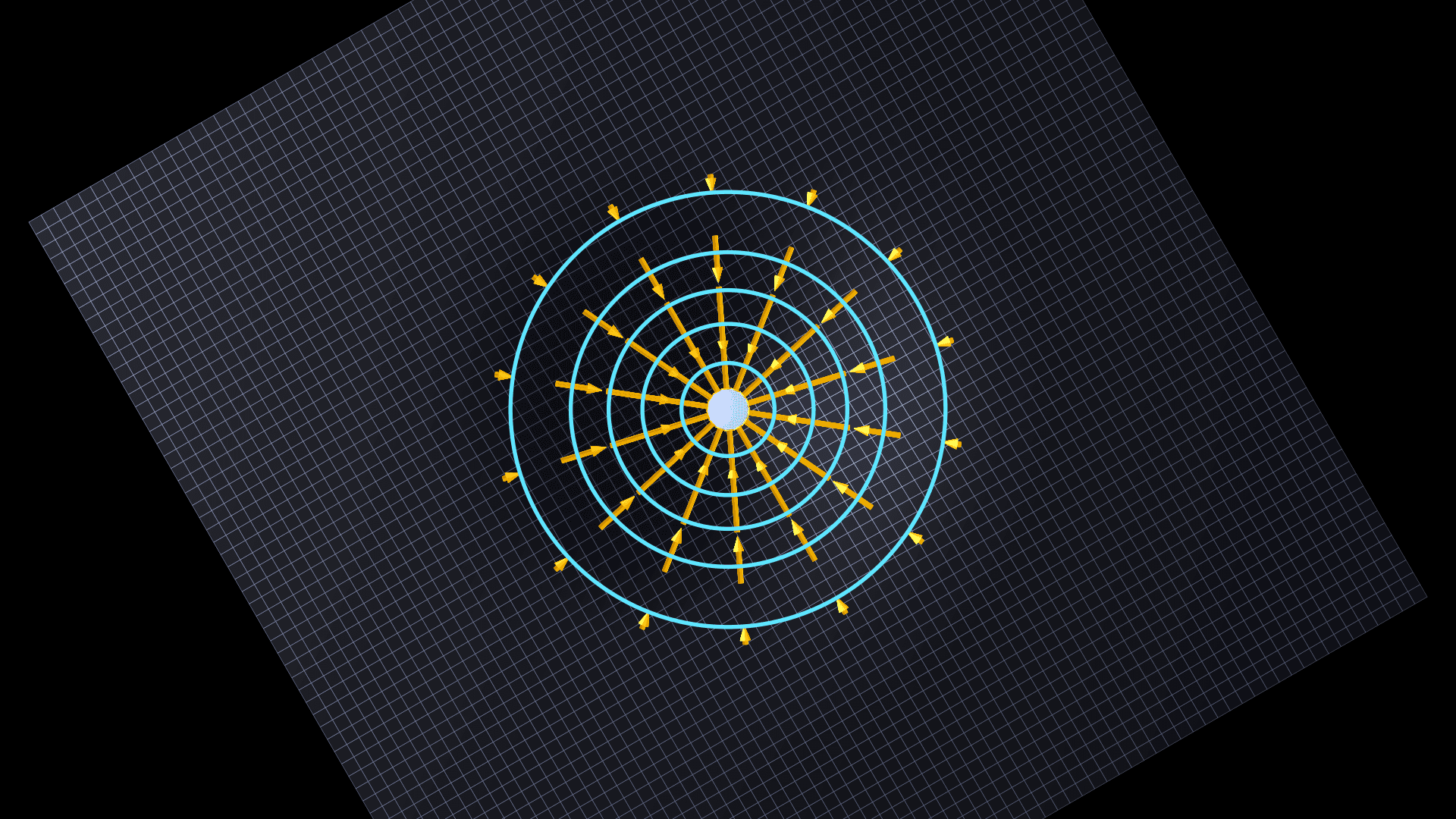
Strictly top-down, the depth disappears and the level sets read as exact concentric circles — a topographic map of the action. The arrows still point along ; from above you can see directly that they are radial inward.
Symmetries of yield conservation laws by Noether's theorem (1918), one of the deepest results in twentieth-century physics: every continuous symmetry of the action implies a conserved quantity. Time-translation symmetry implies energy conservation; space-translation implies momentum; rotation implies angular momentum. The reason "conservation laws" exist as a category at all is that the universe has symmetries.
The quantum step is severe: quantization promotes from a number-valued function to an operator-valued distribution acting on a Hilbert space. A Hilbert space is the abstract list of all possible quantum states of a system — like "every possible configuration of the universe," but organized as a vector space so that states can be added and rescaled. An operator is a rule for transforming states; measuring the field at a point gives a number that depends on which state the universe happens to be in. A "distribution" is a generalization of a function that allows infinitely concentrated values (like a delta function), which is the right object when you ask the field's value at a single mathematical point.
What this means physically is that the field can now create and destroy particles. Every electron in the universe is an excitation of the same electron field, and there is no "this electron" and "that electron" — they are mathematically identical because they are modes of the same underlying operator. Imagine a sheet of fabric stretched across the universe; a small ripple in the sheet, with the right shape, is an electron. There is no factory stamping out electrons; there is one fabric, and the rules of the fabric determine what counts as an electron. This is why every electron has identical mass and charge.
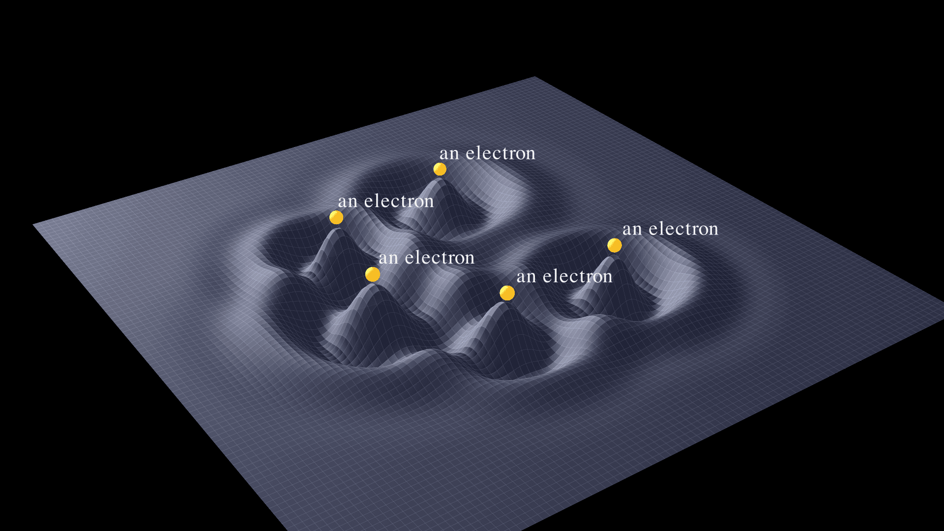
Particles are excitations of fields, not separate objects. The universe has one electron field; every individual electron is a localized ripple in it. Each wave packet here is the same kind of object as every other one — same field, same rules, same mass and charge.
The organizing structure of the quantum theory is the Feynman path integral:
It sums over all possible histories of the field, weighted by a complex phase. Heuristically: in classical mechanics a particle picks one trajectory between two points. In quantum mechanics it tries every trajectory at once, weighting each by . Most trajectories have wildly oscillating and their contributions cancel in pairs; the trajectories whose action is stationary — where — survive because neighboring paths agree in phase and add constructively. Classical physics is the limit where one path dominates so completely that the others vanish. The path integral is therefore not a competitor to least-action; it is why least action holds.
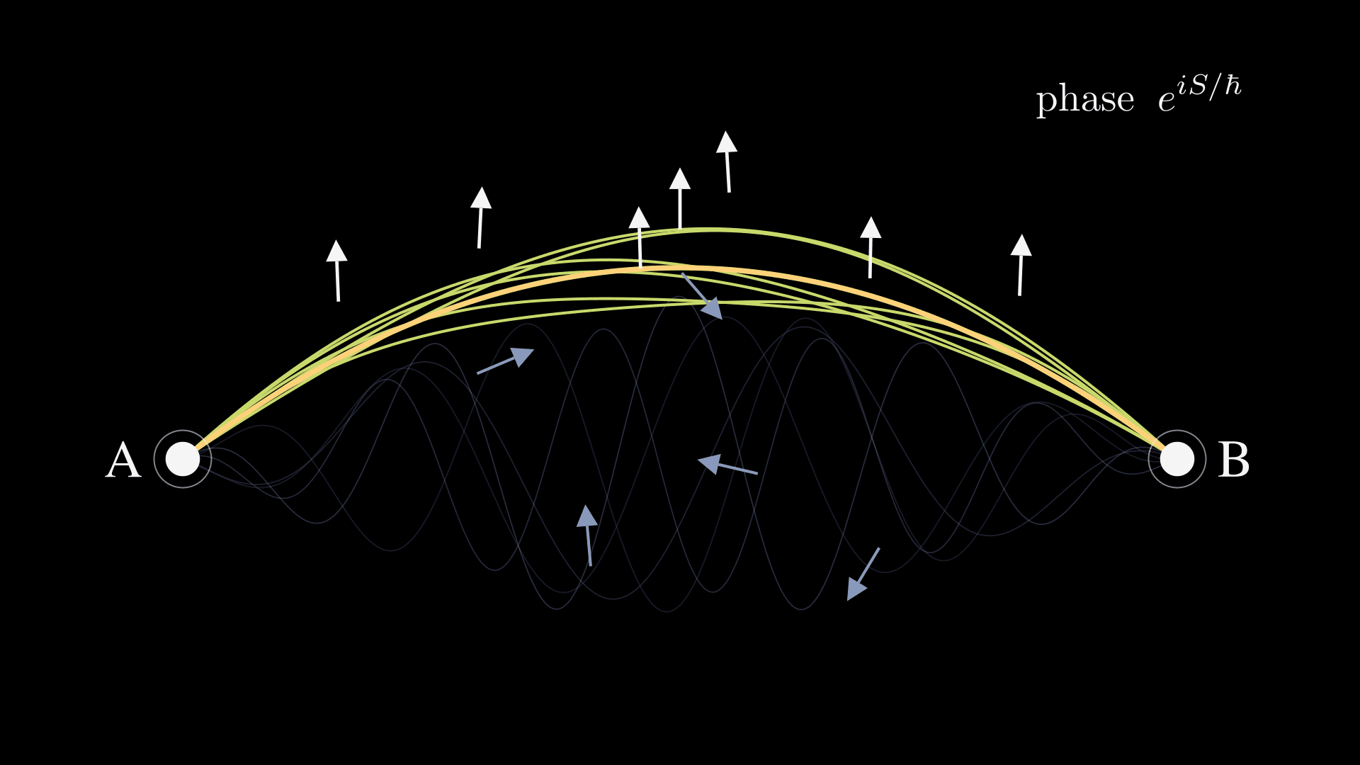
Every trajectory from to contributes a phase to the path integral. Trajectories near the classical path (gold) have nearly the same action , so their phases align and add constructively — the comb of parallel white arrows above the arc. Wild trajectories (blue-gray) have rapidly varying ; their phases scatter around the unit circle and cancel. The classical path is the one whose neighbours agree.
After a Wick rotation to Euclidean time — replacing time by an imaginary parameter , which turns oscillating phases into damped real exponentials — the path integral becomes a statistical partition function, identical in form to the Boltzmann weights of statistical mechanics. A great deal of intuition transfers directly between thermal physics and quantum field theory by way of this rotation.
Three Lagrangians that appear constantly in what follows:
The notation: is the four-derivative — the gradient generalized to spacetime, so is time and are the three spatial derivatives. The are the Dirac matrices, four 4×4 matrices that encode how spinors mix under Lorentz transformations. is the gauge field strength, the curl of the gauge potential . The Klein-Gordon equation governs a free spin-0 scalar, the Dirac equation a spin- fermion, and Yang-Mills a non-abelian gauge field.
Spinors are the geometric objects that fermions live in. Unlike vectors, which return to themselves under a rotation, spinors return to minus themselves and only come back home after . This is not a quirk; it is the algebraic reason fermions obey the Pauli exclusion principle. The Dirac equation is the wave equation that spinors satisfy. A Weyl spinor is half of a Dirac spinor — either the left-handed or right-handed component, with two complex entries each.
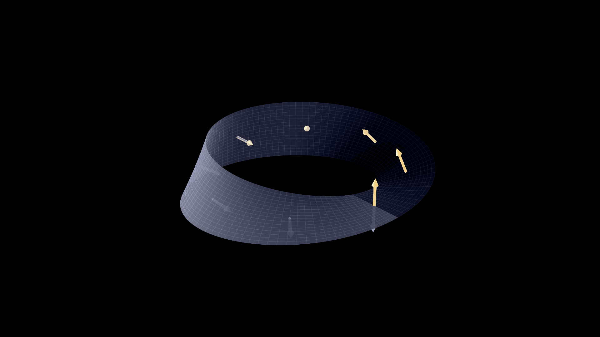
The Möbius strip's half-twist is the geometric content of the SU(2)→SO(3) double cover. An arrow placed on the strip and walked once around its central circle returns to the same physical point, but its orientation has flipped — the spinor's sign change after . Walking around twice (the orientable double cover) restores the original orientation: to come back to itself.
The commutator term hidden inside the Yang-Mills field strength — the part proportional to — is what distinguishes gluons from photons. Photons are electrically neutral; they do not push or pull other photons. Gluons carry color charge themselves, so two gluons can scatter. This self-interaction is what makes the strong force confine quarks at long distances, and what makes non-abelian gauge theory qualitatively different from the abelian case.
A third flavor of field theory, beyond classical and quantum: a conformal field theory (CFT) is one with no preferred scale. Under the rescaling the theory looks the same — zoom in by a factor of two, zoom out by a factor of seventeen, the rules are unchanged. There is no fundamental length, no fundamental energy. Critical points of phase transitions (water at its critical point, magnets at the Curie temperature) are CFTs. The full conformal group in dimensions is , the rotation group of a flat space with time-like and space-like directions (the signature is conventional). It contains Poincaré as a subgroup, plus a dilatation generator that scales and special conformal generators . The relevant commutators:
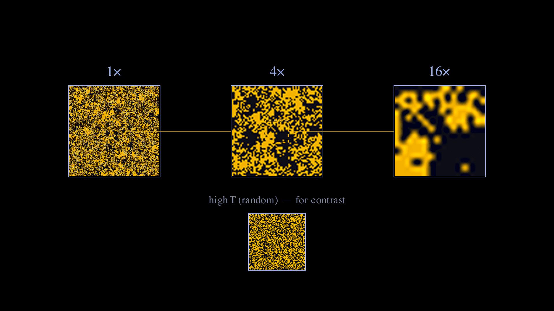
A 2D Ising model at the critical temperature , viewed at three nested magnifications. The cluster structure persists at every zoom level — that is the visual content of conformal invariance: the field has no preferred length scale. The bottom panel shows a snapshot at the same per-cell display resolution; with no spatial correlations, no structure appears at any scale. Critical Ising looks self-similar; high-T noise looks featureless.
CFTs are not exotic edge cases. The renormalization group ("RG") is the rule for how a theory's parameters change as you zoom in or out — what coupling constants and masses look like at the energies your microscope can resolve. Wilson's insight in 1971 was that physics at every scale is a flow in the space of all possible theories: short-distance details get washed out, and theories converge to a small number of universal endpoints called fixed points. CFTs are these fixed points. Every quantum theory you have ever heard of is either flowing toward one or sitting at one. Studying CFTs is studying the attractors of the entire flow.
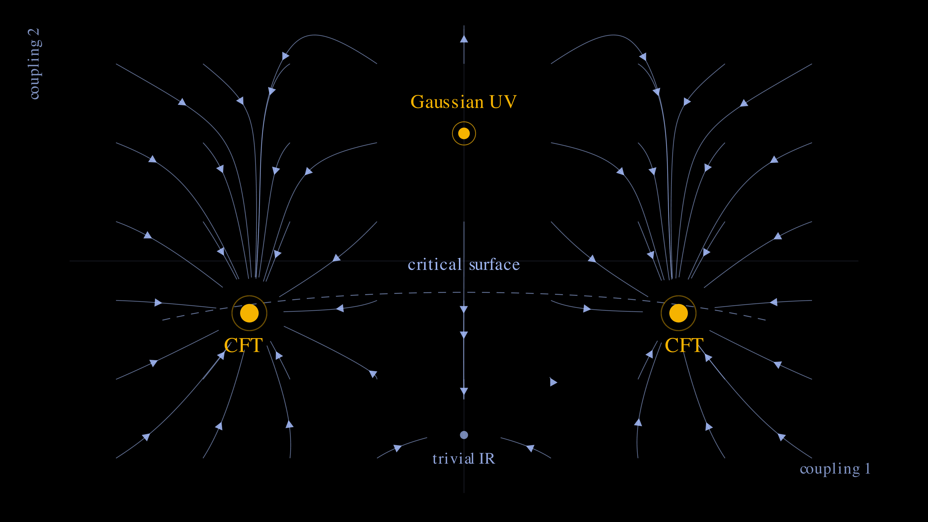
RG flow lines in the space of all theories. Each streamline is the trajectory of a quantum field theory under change of scale. Most theories flow to a fixed point; the fixed points are CFTs (the two amber sinks) or trivial gapped phases (the small blue sink). The dashed line is the critical surface — the codimension-1 set of theories that flow to a CFT instead of becoming gapped. Mathematically the flow is gradient-like: Zamolodchikov's -theorem says there is a function on theory space that decreases monotonically along every flow.
The Standard Model in one breath
The Standard Model is a gauge QFT with internal symmetry group
A few words on what these symbols mean. is the group of unitary matrices with determinant — abstractly, the rotations of an -dimensional complex space. is the simplest Lie group, a circle, parameterized by a single phase. An internal symmetry mixes different fields among themselves at the same spacetime point; it does not move points around the way a rotation does. The Standard Model says: nature is invariant under independent rotations in three abstract internal spaces.
acts on three "color" charges of quarks (red, green, blue — labels, not real colors). is weak isospin, acting on a two-dimensional space mixing left-handed up-type and down-type fermions. assigns a weak hypercharge to each particle. The subscripts , , keep these three factors distinct from any other , , or that might show up. After electroweak symmetry breaking, the unbroken subgroup is — color plus ordinary electromagnetism.
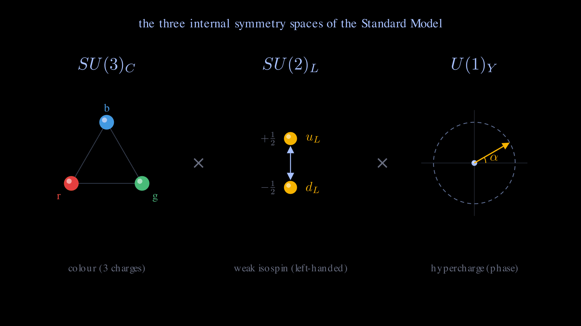
The three internal symmetry spaces of the Standard Model. acts on the three colour charges of each quark; acts on left-handed fermion doublets; is a phase rotation on hypercharge eigenstates. The full SM gauge group is the direct product of all three: .
Fermion content: three generations of quarks and leptons, each generation containing an doublet of left-handed quarks, two right-handed quark singlets, a left-handed lepton doublet, and a right-handed charged lepton. The SM is chiral: left-handed and right-handed fermions transform under different gauge representations. Chirality is handedness: a left-handed fermion has its spin pointing opposite to its momentum; a right-handed one has them aligned. The weak force, alone among the fundamental forces, treats left and right asymmetrically — only left-handed neutrinos appear in the theory, and right-handed ones (if they exist at all) are sterile.
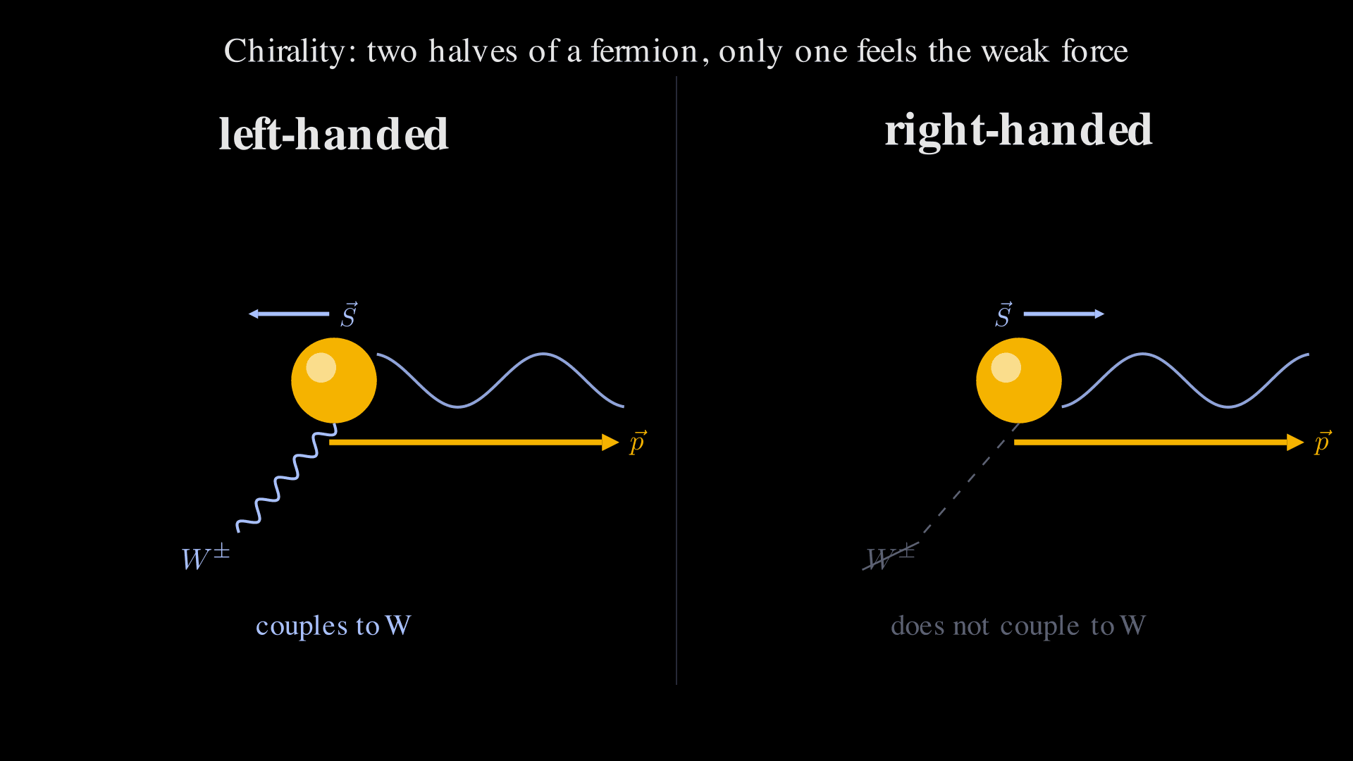
Helicity is the projection of spin along the direction of motion. A left-handed particle has spin antiparallel to its momentum; a right-handed particle has them aligned. The weak interaction couples only to the left-handed component of every Standard Model fermion. For massive particles, chirality (the irreducible Dirac projection that the weak force actually sees) and helicity (the spin-momentum picture above) coincide only in the ultrarelativistic limit, but the helicity picture captures the physical asymmetry well enough for our purposes.
Chirality matters here. A bare fermion mass term mixes fields with different gauge charges, which invariance forbids. The left-handed piece of the fermion carries weak-isospin charge; the right-handed piece does not. Combining them directly is like adding a colored ball to a colorless one and pretending the result is colorless — the combination is not gauge-invariant. Fermion masses therefore cannot be fundamental; they must arise from a coupling to a scalar field that supplies exactly the missing charge to make the combination consistent. That scalar is the Higgs.
The Higgs field and its self-coupling
The Higgs is an doublet of complex scalars, the only fundamental scalar in the theory. Its potential has the Mexican-hat shape:
With and , the origin is a local maximum. The minimum is a ring at .
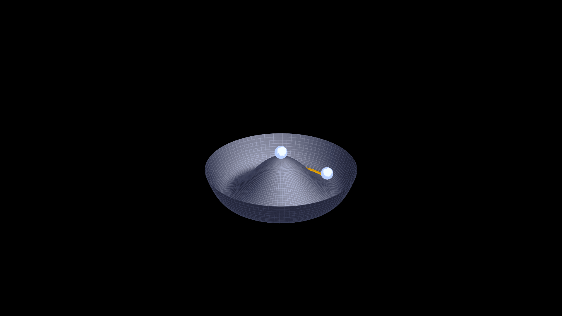
The Higgs potential . The origin is a local maximum (the symmetric, unstable vacuum); the minimum is a circle at . The universe picks one point on the rim — that's spontaneous symmetry breaking. The amber arc traces the Goldstone direction: motion along the rim costs zero energy, so the field has massless modes in that direction. Three of them, in the SM. They are eaten by the and bosons to give those gauge bosons their longitudinal polarisations and masses; only the radial mode (perpendicular to the rim) survives as the physical Higgs.
The universe picks a point on this ring — spontaneous symmetry breaking. Imagine a pencil balanced on its point. The setup is rotationally symmetric; every direction is equivalent. But the pencil cannot stay balanced; it must fall some way, and once it has fallen, the symmetry is broken even though the laws of physics remain symmetric. The Higgs vacuum does the same thing: the laws are symmetric under , but the actual ground state of the universe sits at one specific point on the rim of the Mexican hat, and that choice gives mass to the W and Z bosons. The vacuum expectation value (VEV) — the quantum-statistical average of the field over the empty vacuum, like a permanent background field permeating all space, but for weak charge rather than electromagnetism — is
The value GeV is not a free parameter; it is fixed by the precisely measured Fermi constant. The Higgs doublet starts with four real scalar fields. Three of them become Goldstone modes — massless excitations along the rim of the hat, which cost no energy because the rim is a flat valley. The Higgs mechanism (Brout-Englert-Higgs, 1964) absorbs these Goldstones into the gauge bosons: a massless gauge boson has 2 polarization states, a massive one has 3, and the Goldstone provides the missing third. The fourth scalar, the radial direction climbing out of the rim, is the physical Higgs particle that ATLAS and CMS discovered. The W and Z masses are
Fermion masses come from Yukawa couplings. A Yukawa coupling (after Hideki Yukawa, who introduced this kind of interaction in 1935 to model the nuclear force) is a three-way interaction term in the Lagrangian binding a fermion, an antifermion, and a scalar:
When the scalar takes its VEV , the term collapses into an ordinary mass term with
The Yukawa coupling sets how strongly each fermion interacts with the Higgs, and therefore how heavy it is. The top quark, with , is the heaviest particle at GeV. The electron, with , is 511 keV. That's six orders of magnitude in Yukawa couplings with no explanation — the flavor puzzle, adjacent to but distinct from what we are about to discuss.
The surviving scalar excitation around the vacuum, the physical Higgs boson , has mass
ATLAS and CMS announced the discovery of a boson at GeV on 4 July 2012 (arXiv:1207.7214, arXiv:1207.7235). Each collaboration reached independently. The current PDG average is GeV, which gives
This value of matters beyond the tree-level mass. Running a coupling means asking what its effective value would be in scattering experiments at energy , after summing up all virtual quantum effects from energies between and the renormalization point — concretely, this is RG flow applied to a single number. The Higgs self-coupling depends on ; at low energies it is positive (stable Mexican hat), but a two-loop calculation shows it crosses zero somewhere around – GeV. A negative quartic means the Mexican hat tilts: a deeper vacuum exists at enormous field values, and the universe is therefore metastable. Metastable means we live in a local minimum of the potential, but a deeper minimum exists somewhere else, separated by a barrier. Quantum tunneling can take a region of the universe from our vacuum to the deeper one; if it does, a bubble of true vacuum expands at the speed of light, and inside the bubble the laws of physics are different. The estimated tunneling rate is many orders of magnitude longer than the age of the universe, but it is finite. Buttazzo et al. (arXiv:1307.3536) describe the SM as living at "near-criticality" between absolute stability and instability. Whether this is a hint of new physics or an accident is unknown.
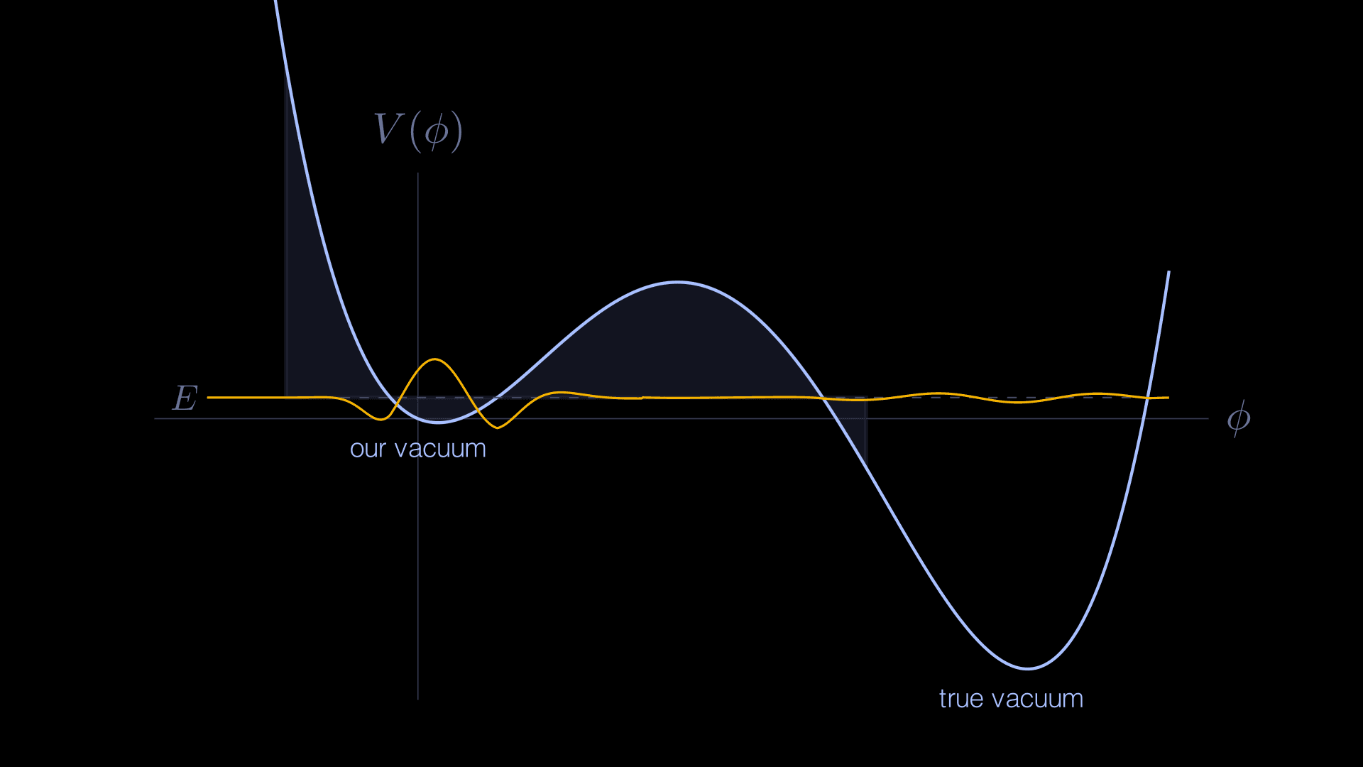
We live in a local minimum of the Higgs potential. Somewhere else in field space — at values where has run negative, around – GeV — is a deeper one. Quantum tunneling can take a region of the universe from our vacuum to the true vacuum, after which a bubble of true vacuum expands at the speed of light. The tunneling rate is far longer than the age of the universe, but finite. The amber wavefunction's small oscillation in the right-hand well is the tunneling tail.
Measuring directly requires producing two Higgs bosons in a single collision. Di-Higgs production is rare and backgrounds are severe. ATLAS and CMS have placed limits ( at 95% CL from ATLAS; similar from CMS, where ) but have not yet resolved at the few-sigma level. The HL-LHC, with 3000 fb, should get to roughly precision; a future 100 TeV collider could pin it to a few percent.
The hierarchy problem
The Higgs is the only fundamental scalar in the SM. Every other particle either has a mass protected by a symmetry or is massless for a structural reason. Gauge bosons are massless because of gauge symmetry; their masses after EWSB track the VEV . Fermion masses are protected by chiral symmetry: setting enhances the symmetry of the Lagrangian (left- and right-handed rotations decouple), so radiative corrections to are proportional to itself, at most logarithmic in the cutoff.
Scalars have no such protection. 't Hooft's naturalness criterion (from his 1980 Cargèse lectures) states: a parameter is natural if setting it to zero enhances the symmetry of the theory. Why should this matter? Take the electron mass as a worked example. If we set , then left-handed electrons no longer mix with right-handed electrons via the mass term, and the two decouple — the theory acquires a new chiral symmetry rotating left and right independently. Symmetries protect zeros: if a symmetry forbids any nonzero value at , then radiative corrections must also vanish there, and any actual nonzero can only generate corrections proportional to itself — logarithmic in the cutoff, not quadratic. For the Higgs, no symmetry appears when ; nothing is enhanced by the limit, and so nothing protects it.
Radiative corrections to are therefore proportional to the cutoff squared:
Two pieces of notation. is a cutoff: the highest energy scale at which the theory is trusted, beyond which we expect new physics. The minus sign on fermion loops is a fundamental quantum-statistical fact: a closed loop of fermions counts with relative to a closed loop of bosons, traceable back to the spin-statistics theorem. This is the reason SUSY can cancel divergences between bosons and fermions — the signs are forced.
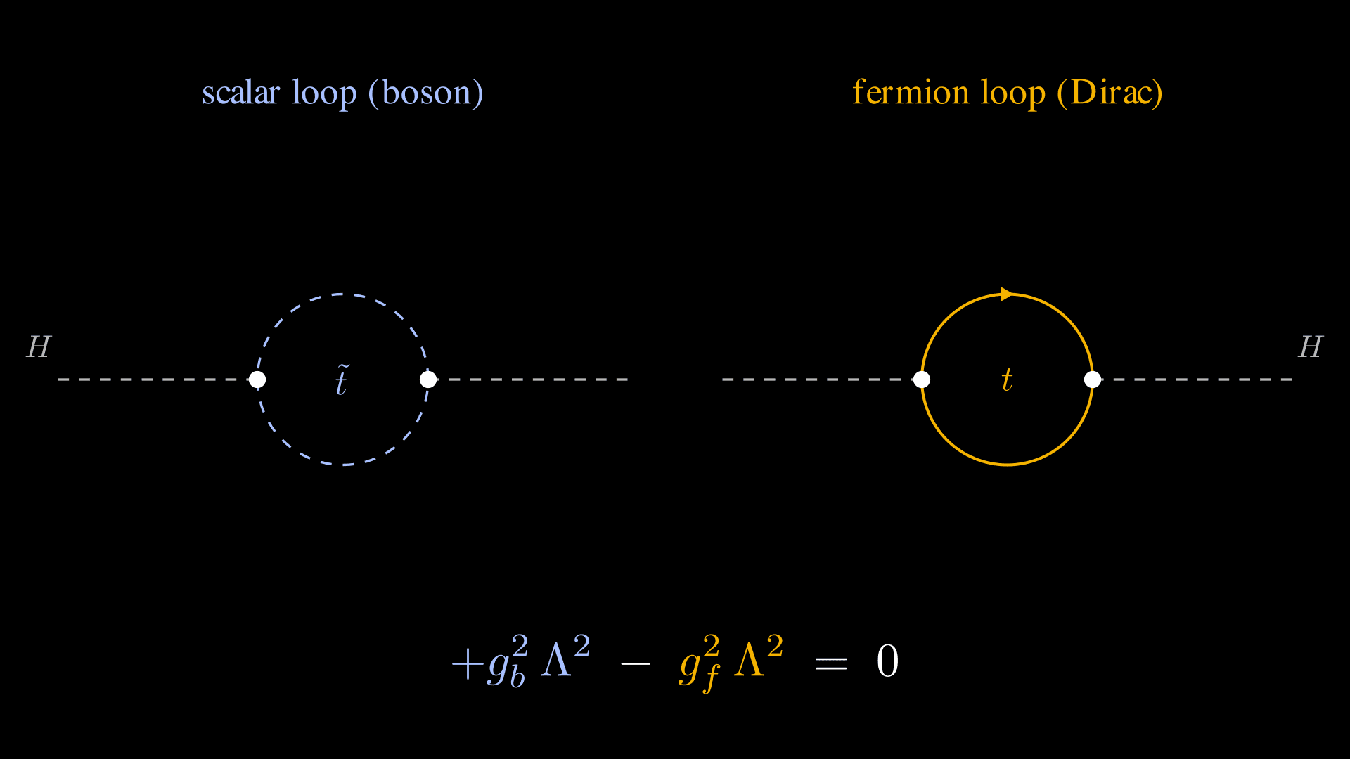
The Higgs self-energy receives a quadratically divergent correction from each scalar in the loop, and from each Dirac fermion. The minus on the fermion is the closed-fermion-loop sign, a Feynman-rule consequence of Fermi-Dirac statistics. SUSY pairs every Standard Model fermion with a scalar superpartner of equal coupling — when , the two contributions cancel exactly, leaving the Higgs mass natural at the cutoff.
The dominant contribution is the top-quark loop, with Yukawa coupling :
If is the Planck scale GeV (the energy at which gravity becomes as strong as the other forces and quantum fluctuations of spacetime itself can no longer be ignored — the natural ceiling for any QFT that does not include quantum gravity), then GeV. The physical value is GeV. The bare mass and the quantum correction must cancel to one part in .
This is not a mathematical inconsistency. The SM works fine if you simply impose GeV by fiat. The discomfort is that nature appears to have set two enormous numbers to cancel almost exactly, with no explanation of why. It looks like a cancellation that should have an underlying reason. Finding that reason, or accepting that none exists, is the hierarchy problem.
Enter supersymmetry
Notice the sign in the loop formula. Bosonic loops and fermionic loops contribute with opposite signs: a closed fermion line picks up a factor of relative to a boson loop. If every SM boson had a fermionic superpartner with identical gauge quantum numbers and identical coupling strength, and vice versa, the quadratic divergences would cancel exactly:
The canonical example is the top quark and its scalar superpartner, the stop . The top contributes . SUSY forces the stop's coupling to equal , so the stop contributes . They cancel:
In exact SUSY there is no quadratic divergence. In softly broken SUSY (the real world, since we obviously do not observe selectrons and squarks at the same mass as electrons and quarks), the residual correction is , logarithmic only. If stop masses are near a TeV, the fine-tuning is manageable.
A note on naming. SUSY's convention is mechanical: each SM fermion gets a scalar partner with an "s-" prefix (selectron, squark, sneutrino), and each SM boson gets a fermion partner with an "-ino" suffix (photino, gluino, higgsino, wino, zino). Collectively the partners are sparticles. The tilde notation marks the scalar top (the stop); is the gluino; and so on.
The first 4D supersymmetric field theory was written down by Gol'fand and Likhtman at the Lebedev Institute in 1971, extending the Poincaré algebra by anticommuting spinor generators. The paper was known only in Russian for years. Volkov and Akulov (1972) independently discovered nonlinearly realized SUSY. Wess and Zumino (1974, Nucl. Phys. B70) wrote the first interacting linearly-realized 4D SUSY field theory, which put SUSY on the Western physics radar. The Minimal Supersymmetric Standard Model was constructed by Dimopoulos and Georgi in 1981 (Nucl. Phys. B193). It adds, to the SM particle content: a gaugino (fermion) for each gauge boson, a squark/slepton (scalar) for each fermion, and two Higgs doublets instead of one. After electroweak symmetry breaking, the electroweak gauginos (bino, winos) mix with the higgsinos (the fermionic partners of the two Higgs doublets) to form four neutralinos and two charginos in the mass basis. A conserved -parity makes the lightest superpartner stable — the LSP, the dark-matter candidate.
Beyond naturalness, SUSY has two other original motivations worth naming. Adding the MSSM particle content, the three SM gauge couplings run with energy and meet at a common scale GeV. This is gauge coupling unification, first sharpened with LEP-I data in 1991. And with a conserved -parity, the lightest superpartner is stable and has the right relic abundance to account for dark matter.
The algebra: SUSY as the square root of translations
That SUSY cancels quadratic divergences is a consequence of algebraic structure, not coincidence. To see why it must take this form, we need a theorem and its loophole.
Coleman and Mandula in 1967 asked: how much can we extend the symmetries of relativistic physics? Their answer was a no-go theorem. Under reasonable assumptions, no Lie-algebraic extension of Poincaré symmetry can mix nontrivially with spacetime structure. You can add internal symmetries (like ), but they sit next to the Poincaré algebra, not entangled with it.
Under mild assumptions (interacting relativistic QFT in , finitely many particle types per mass, and a nontrivial -matrix), the most general bosonic symmetry algebra of the -matrix is a direct product , where internal generators are Lorentz scalars commuting with momentum.
The -matrix — for "scattering" — is the function that takes incoming particles to outgoing particles in a collision experiment; it is the experimentally measurable content of a relativistic QFT. The theorem kills attempts to unify spacetime and internal symmetries in a single Lie algebra. The intuition: Poincaré already pins down the kinematics of two-body scattering up to the angle, and adding more bosonic generators would over-constrain and force the amplitude to vanish except at isolated angles, contradicting analyticity.
The theorem assumes ordinary Lie algebras whose generators satisfy commutation relations. The single loophole: what if some generators anticommute?
The most general symmetry algebra of a nontrivial 4D -matrix, allowing for super Lie algebras graded by even/odd parity (where odd generators anticommute with each other and commute with even ones), is the super-Poincaré algebra, possibly with central charges, plus an internal bosonic algebra.
This isn't an aesthetic preference. HLS says that if you want any extension of Poincaré symmetry at all, it must be supersymmetric. The new generators and their conjugates must be spin- Weyl spinors — recall, half of a Dirac spinor, two complex components. The undotted index labels left-handed components; the dotted index labels right-handed; the difference is a matter of conjugate representations of , the double cover of the Lorentz group. Their defining relation is
The right-hand side is , twice a momentum generator. Applying a SUSY transformation twice equals a translation. The supercharge is, in the most literal sense, a square root of translation, just as the Dirac operator is the square root of the wave operator .
With sets of supercharges, the algebra extends to
The central charges are extra commuting bosonic generators — "central" in the group-theoretic sense that they commute with everything. Antisymmetry in means vanishes identically for ; central charges only exist in extended SUSY, . Physically they show up as quantized BPS masses: a particle's mass is bounded below by its central charge, and saturation of that bound defines the BPS states (Bogomol'nyi-Prasad-Sommerfield) — particles whose masses are protected from perturbative corrections, making them ideal probes of strong-coupling physics. Central charges become load-bearing in Seiberg-Witten theory and BPS state counting.
Two senses of extra dimensions
Here is the point the title is gesturing at. "Extra dimensions" in physics usually calls to mind Kaluza-Klein scenarios: curled-up spatial dimensions too small to see. SUSY gives us two conceptually distinct instances of new dimensions, only one of which is spatial.
Superspace: fermionic extra dimensions
The SUSY algebra poses an immediate geometric puzzle. The generators are spinors, not vectors, and they do not generate any motion on ordinary spacetime — there is nowhere for them to "act" geometrically. They square to translations, but they themselves must anticommute.
The resolution, due to Salam and Strathdee in 1974, is to extend spacetime by adjoining new anticommuting coordinates. The superspace in 4D has coordinates
The 's are Grassmann numbers: , in particular . Superspace is a supermanifold of dimension . The vertical bar separates ordinary bosonic coordinates from anticommuting fermionic ones: bosonic plus fermionic. The two halves are not added in the way real dimensions are; no inner product mixes them, and the notation is a bookkeeping device for keeping track of how many of each kind you have.
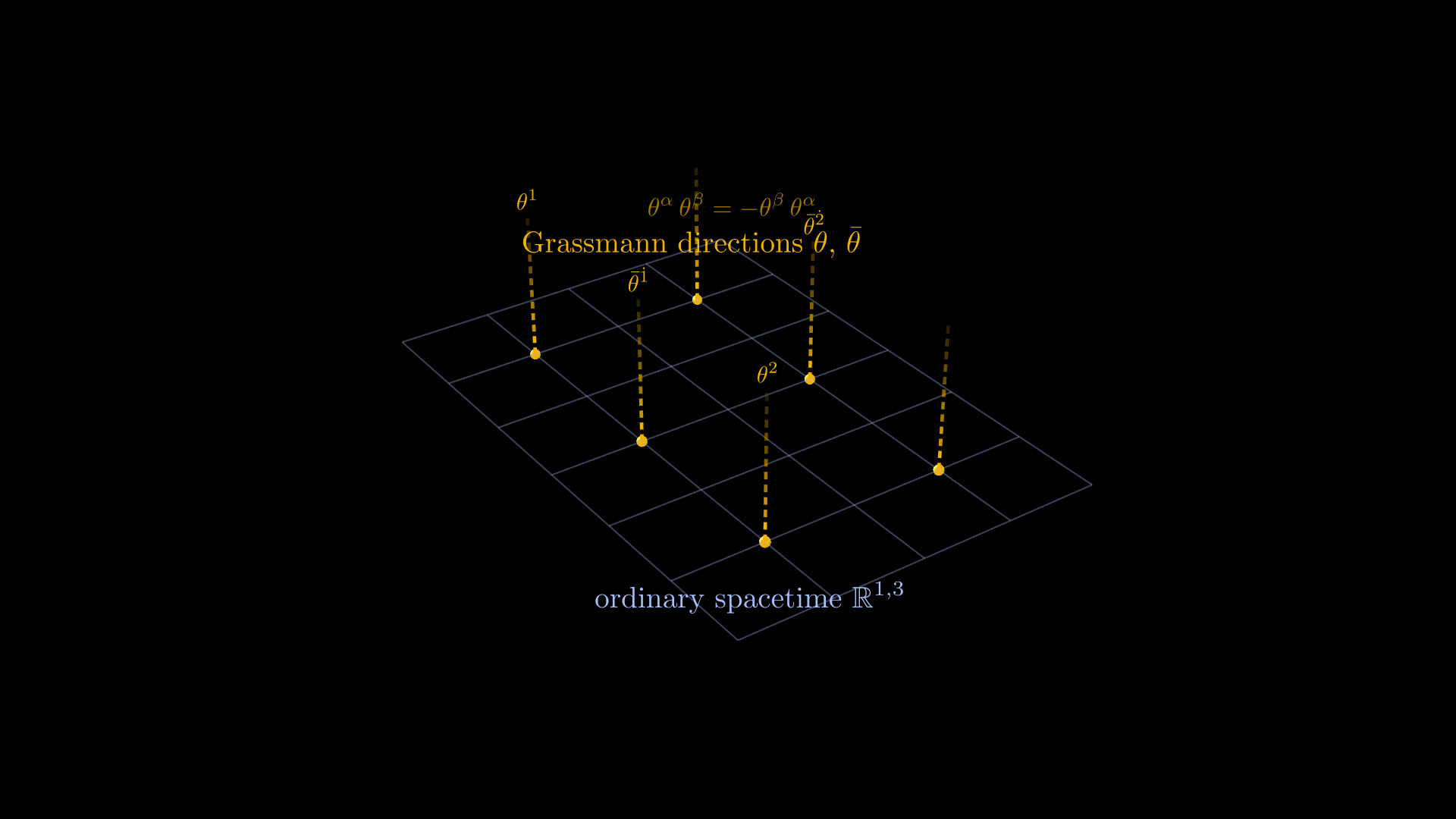
Superspace as a fiber bundle. The base is ordinary spacetime . Attached at every point is a four-dimensional Grassmann fiber spanned by . The fibers fade out of geometric reality because the 's aren't real-valued coordinates — they anticommute and square to zero, . Superspace = spacetime with anticommuting fibers attached at every point.
A superfield is a function on superspace, . Because , the Taylor expansion in , terminates after finitely many terms. Imposing a chirality constraint gives a chiral superfield. Here is the superspace covariant derivative — a derivative that anticommutes with the supercharge instead of commuting with it. The constraint is the SUSY analog of holomorphy: it picks out "left-moving" superfields the way picks out holomorphic functions on the complex plane. The component expansion is
Just three lines, and yet expanding them reveals a complete supersymmetric multiplet: is a complex scalar, a Weyl fermion, and an auxiliary scalar — a field with no kinetic term and no independent particle interpretation, integrated out via its algebraic equation of motion to leave extra interactions among the physical fields. Auxiliary fields close the SUSY algebra off-shell; once you eliminate them, the surviving Lagrangian still has SUSY, but the algebra needs the equations of motion to close.
Their couplings, masses, and interactions are all fixed by the single holomorphic superpotential . Holomorphic means: depends on the chiral superfield but not its complex conjugate — analogous to a complex-analytic function rather than . SUSY forces this restriction, and it is the technical reason many quantities in SUSY theories can be computed exactly. The Wess-Zumino action
with expands to many pages of component-field action: kinetic terms, Yukawa couplings, and a quartic scalar potential, all dictated by SUSY. To taste the mechanics: the kinetic part expands to . A single superspace integral knows about both the scalar's and the fermion's kinetic terms, and even hands you the auxiliary for free. Every Yukawa coupling in the component theory comes from a derivative of . Get right and the rest is mechanical. This is the "strong type system" aspect: write the theory on superspace, and the compiler infers the rest.
The four fermionic coordinates are the extra dimensions that SUSY requires. They are not spatial. They are anticommuting, algebraic, real in the sense that fields must be sections of bundles over the supermanifold. The SUSY algebra cannot be realized on ordinary spacetime alone; it needs this extended geometry.
Spatial extra dimensions: strings and M-theory
The second sense is the familiar one. Consistent supersymmetric string theories exist only in 10 spacetime dimensions. M-theory, their strong-coupling limit discovered by Witten in 1995, lives in 11. To make contact with our 4D world, you compactify the extra dimensions on a small compact manifold of dimension .
The topology and holonomy of control how much SUSY survives. Holonomy of a Riemannian manifold is the group of rotations a vector can pick up by being parallel-transported around a closed loop. Generic -manifolds have holonomy; manifolds with extra structure have smaller holonomy groups, and the smaller the group, the more covariantly constant spinors the manifold admits — and each such spinor preserves one supersymmetry in the lower-dimensional theory.
- Compactify on a torus : holonomy is trivial, all 32 supercharges survive, giving 4D . Too much symmetry for phenomenology — there is no chirality.
- Compactify heterotic string theory on a Calabi-Yau threefold (Candelas-Horowitz-Strominger-Witten 1985): get 4D , just enough SUSY for the hierarchy problem. A Calabi-Yau is a six-real-dimensional manifold (three complex dimensions) that is Kähler (its complex and metric structures are compatible) and Ricci-flat (its trace curvature vanishes). The defining geometric property is holonomy. The simplest examples are the quintic in and products like . The reason in 4D survives: a Calabi-Yau admits a single covariantly constant spinor, and every other spinor is rotated by the holonomy as it moves around the manifold.
- Compactify M-theory on a -holonomy 7-manifold: again 4D . The exceptional Lie group has dimension 14 and sits inside ; it is the holonomy group that admits a single covariantly constant spinor in seven dimensions, the analog of in six.
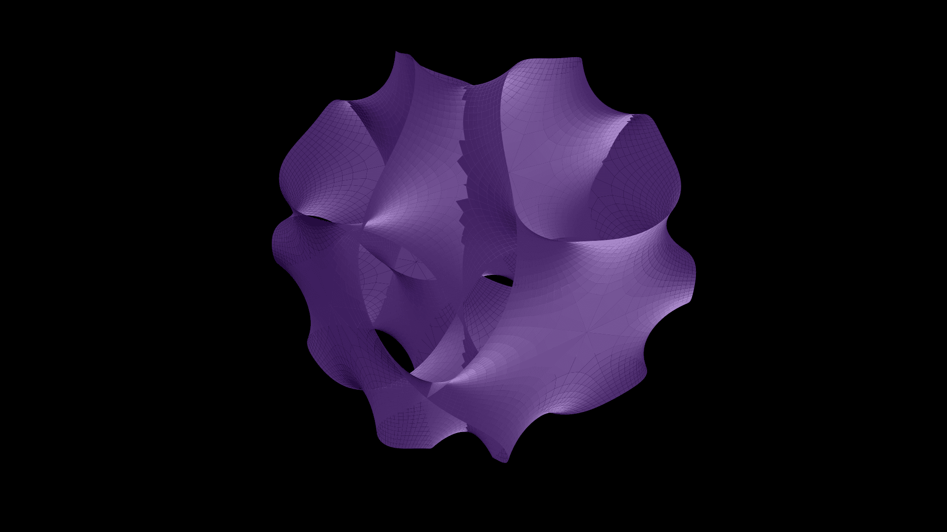
A 2D real cross-section of the Fermat quintic Calabi-Yau threefold, in , projected from to via Hanson's canonical viewing angle. The actual Calabi-Yau is six-real-dimensional and Ricci-flat Kähler with holonomy — exactly the geometry that leaves SUSY in 4D after compactifying heterotic string theory on it.
Each 10D field decomposes into a Kaluza-Klein tower of 4D fields with masses , where is the compactification radius. The mechanism is straightforward: a wave on a small circle has quantized momentum , and that momentum becomes mass from the 4D point of view. Only the mode is light at low energies; the higher modes are stratified above the mass gap .
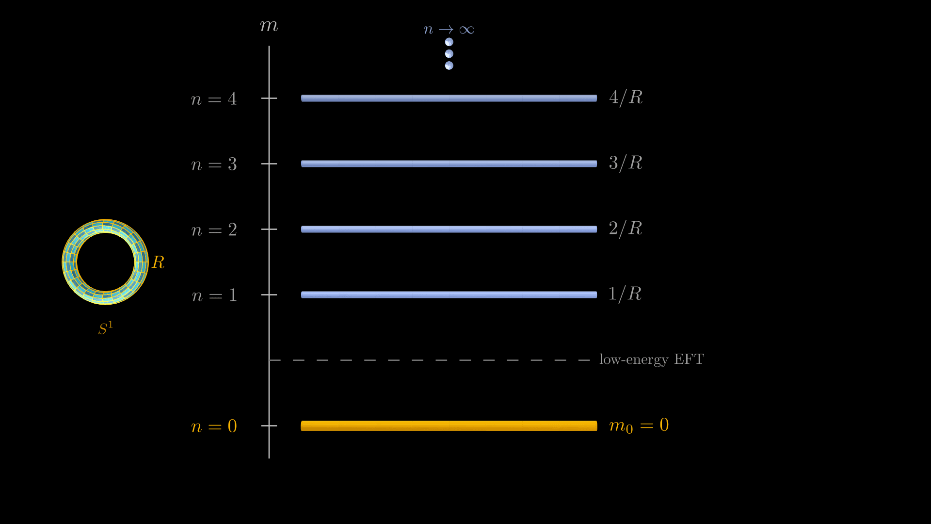
Compactifying on a circle of radius produces an infinite tower of 4D particles with quantized masses . Only the zero-mode is light; the rest decouple if is small. The threshold line marks the boundary of the low-energy effective theory.
These spatial extra dimensions are real, extended directions, not algebraic constructs. They are also conceptually independent of superspace. A superstring theory has both: the string propagates in 10 spatial dimensions (some compact), and the worldsheet theory has fermionic coordinates reflecting the SUSY of the target space. Both notions of "extra dimension" coexist.
Conformal and superconformal symmetry
Adding scale invariance to the Poincaré group yields the conformal group . The generator measures the scaling dimension of an operator. Every quantum field has a scaling dimension — a real number specifying how its expectation value transforms under zooming. A free scalar in 4D has ; a free fermion has . Interactions can shift dimensions to non-rational anomalous values, and the spectrum of operator dimensions is one of the principal observables of a CFT. An operator of dimension transforms under as
The special conformal generators act as "inversion-translation-inversion." The algebra closes on the Poincaré generators via
Combine the conformal algebra with SUSY supercharges and their conformal images (introduced by rotating into something new), and you get a superconformal algebra. In any dimension, the superconformal algebra contains the conformal group, the SUSY algebra, and an R-symmetry group rotating the supercharge index. R-symmetry (the "R" is for Raymond) is an internal symmetry that does not commute with the supercharges; it rotates them into each other, and with supercharges the maximal R-symmetry is .
The natural question: in which dimensions can this structure exist?
Simple Lie superalgebras whose bosonic part contains for some (that is, superconformal algebras) exist only for . For , no superconformal algebra exists.
Six is the hard ceiling. The reason is representation-theoretic: the spinor representations grow with dimension, and past there is no consistent way to fit spinor-valued supercharges inside a finite-dimensional superalgebra containing . The dimensions each support specific superconformal algebras: in 3D, (or for ) in 4D, and in 6D.
Nahm's theorem is why 6D has special status. It is the highest dimension supporting superconformal field theories at all, and the 6D theories are the most constrained and the most mysterious.
The canonical SCFT: SYM in 4D
The "harmonic oscillator of QFT." Every theorist who works with SCFTs has super-Yang-Mills internalized as a benchmark, a test case, and a source of intuition.
The field content, all in the adjoint representation of the gauge group (typically ). The adjoint representation of is the action of the group on its own Lie algebra; for this is an -dimensional space. Gluons in QCD live in the adjoint of , so they come in eight types — the generators of .
- One gauge field (2 on-shell bosonic degrees of freedom)
- Six real scalars , (6 bosonic d.o.f.)
- Four Weyl fermions , (8 fermionic d.o.f.)
The on-shell boson count (8) equals the fermion count (8), as SUSY requires. The symmetry group is , where the R-symmetry rotates the six scalars and (in its fundamental representation) the four fermions. The full superconformal algebra is , with 16 Poincaré supercharges plus 16 conformal supercharges.
The Lagrangian, schematically:
The scalar potential has flat directions when the scalars commute. These are the Coulomb branch vacua. Branches of vacua are connected components of the space of zero-energy field configurations. The Coulomb branch is named for the long-range force surviving when the gauge group is broken to its abelian subgroup — by analogy with electromagnetism, which is the unbroken of the SM after EWSB and gives Coulomb's law. On the Coulomb branch the scalars acquire VEVs and the gauge group is partially broken.
The defining property of SYM: the beta function vanishes to all orders in perturbation theory,
The beta function is the rate of running — the derivative of a coupling with respect to log-energy: . A nonzero beta function means the theory looks different at different energy scales (the SM has for all three of its gauge couplings); a vanishing beta function is the signature of a CFT. The one-loop cancellation between gauge-boson, fermion, and scalar contributions in SYM is forced by the matter content. All-orders vanishing follows from non-renormalization theorems combined with conformal invariance. The theory is conformally invariant for every value of . Nothing runs, no Landau pole appears, and the theory has no preferred scale.
The complexified coupling is believed to be exactly invariant under the duality group:
is the group of integer matrices with determinant ; geometrically it is the symmetry group of the upper half-plane parameterizing complex-structure shapes of a torus. The two generators correspond to twisting the torus by one full cycle () and swapping its two cycles (). The fact that SYM has exactly this symmetry on its complexified coupling is the strongest hint that there is a torus hiding somewhere in its definition — and indeed there is, via the M5-brane realization of SYM as the 6D theory on a torus.
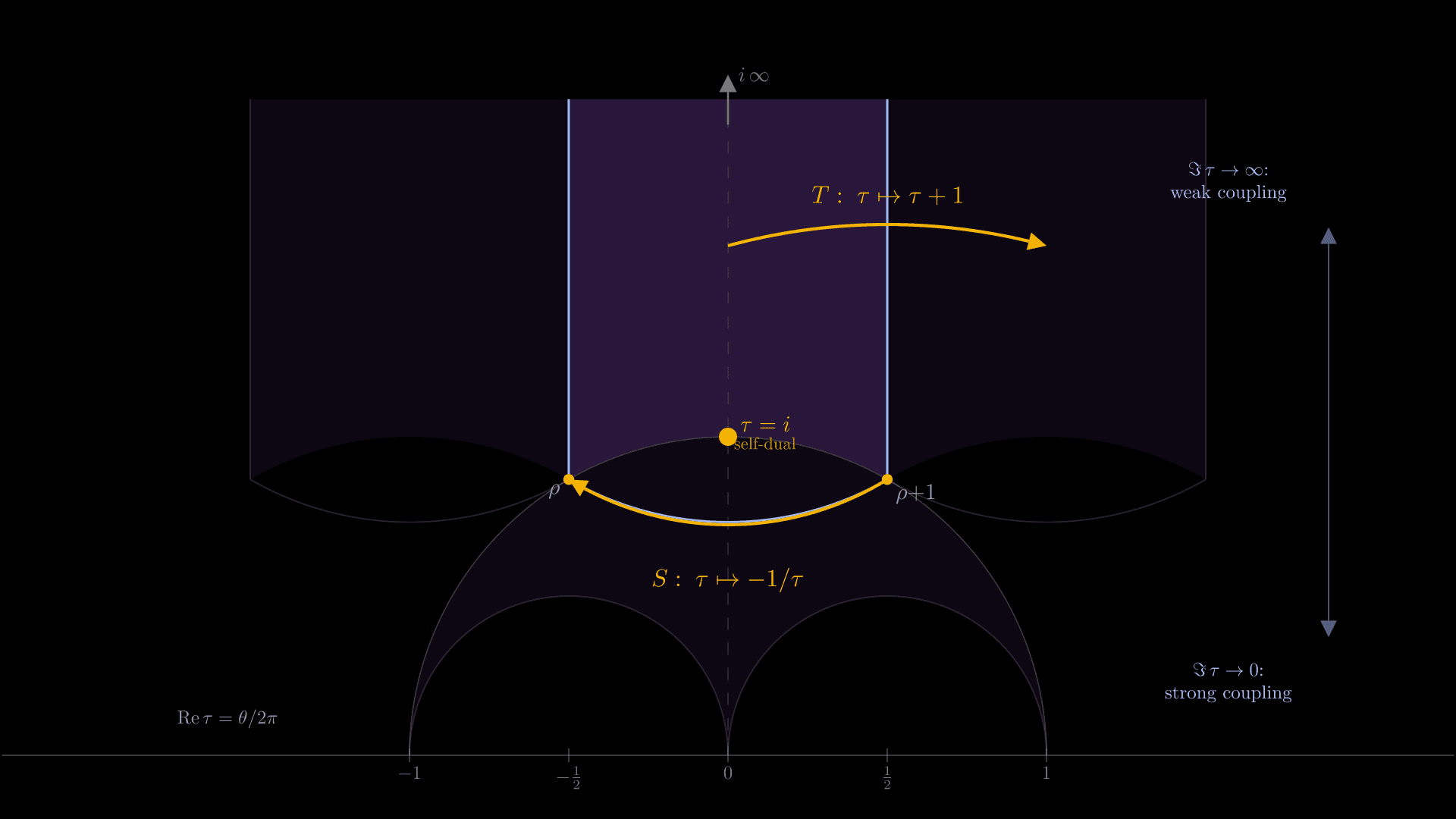
The modular group acts on the complexified gauge coupling . The shaded fundamental domain is the moduli space of physically distinct SYM theories. The generator shifts the theta angle by ; is electric-magnetic duality, fixing the self-dual point and swapping weak and strong coupling. SYM is invariant under all of it.
The first transformation is electric-magnetic duality, exchanging the gauge group with its Langlands dual and swapping weak and strong coupling. The Lie algebra is self-dual, but the global form is not: the Langlands dual of is . The distinction is invisible at the level of local operators but governs the spectrum of extended ones — a Wilson line in the fundamental of maps to an 't Hooft line in . Strong coupling in one global form is weak coupling in its dual.
This S-duality has been used as a workhorse: extracting strong-coupling data from weak-coupling calculations, deriving exact results in integrable subsectors, and (via topological twisting) establishing the geometric Langlands program.
The mysterious one: the 6D theory
The highest-dimensional superconformal theory on Nahm's list is in six dimensions, with supersymmetry. The notation refers to chiral spinors in 6D and indicates 16 left-handed supercharges and none right-handed; physically, this is the worldvolume theory on a stack of M5-branes in M-theory.
No Lagrangian for this theory has ever been written down. There are arguments that none can exist. The theory contains a self-dual 2-form gauge field with satisfying . A 2-form gauge field is the higher-form generalization of the photon potential : where couples to charged point particles, couples to charged strings. Its field strength is the 3-form . Self-duality — the field strength equals its Hodge dual — is an unusual condition that has no covariant Lagrangian formulation, which is part of why no Lagrangian exists for the 6D theory. Various formalisms (PST and others) can handle the self-duality, but none produces a clean, useful Lagrangian.
Despite having no Lagrangian, the theory is unambiguously defined by its symmetry algebra and operator data. It has the superconformal algebra with R-symmetry . The interacting theories are labeled by simply-laced Lie algebras:
- Type : M5-branes in flat space
- Type : M5-branes near a orientifold
- Types : via further M-theory geometry
The ADE classification is a list of three infinite families (, ) and three exceptional cases () of simply-laced Lie algebras, equivalent to a list of finite subgroups of , equivalent to a list of certain singular points on complex surfaces. The same list shows up in du Val singularities, simply-laced Dynkin diagrams, and minimal modular invariants of 2D CFT. The recurrence — the McKay correspondence — has been called one of the deepest unsolved patterns in mathematics. Its appearance throughout mathematics is not coincidental.
In 2009, Gaiotto (arXiv:0904.2715) showed that compactifying the 6D theory of type on a punctured Riemann surface produces a 4D superconformal field theory. Different pants-decompositions of the surface give different Lagrangian descriptions of the same 4D theory, automatically related by S-dualities. Strongly coupled 4D SCFTs with no known Lagrangian description appear naturally as for special curves . The 6D theory with no Lagrangian engineers 4D theories with no Lagrangian, and reveals their dual descriptions along the way.
AdS/CFT: the holographic extra dimension
In November 1997, Juan Maldacena posted hep-th/9711200, now the most-cited paper in high-energy theory. The conjecture:
The 4D superconformal field theory lives on the boundary of a 5D anti-de Sitter space; Type IIB strings propagate in the 10D bulk . Anti-de Sitter space is the maximally symmetric solution of Einstein's equations with negative cosmological constant. is a hyperboloid embedded in flat space — Lorentzian signature forces two time-like directions in the embedding, not one. It has constant negative curvature, like a saddle, in every direction. The isometry group is , which is exactly the conformal group of the -dimensional boundary CFT — for , matches the conformal group of 4D Minkowski space, and the matching is the kinematic spine of the duality. Crucially, AdS has a boundary at infinity: light reaches the boundary in finite time and can bounce back. This boundary is where the dual CFT lives.
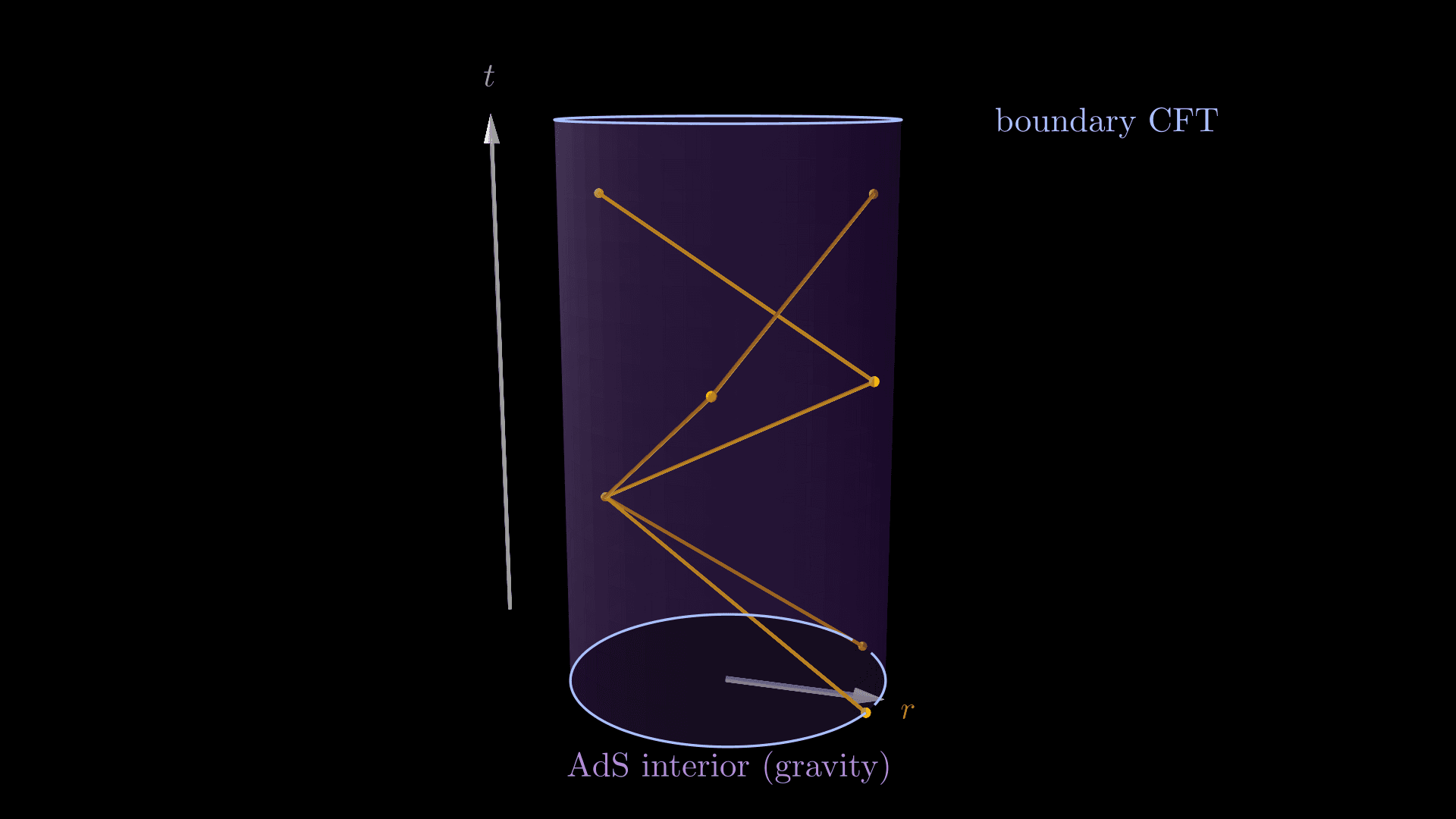
AdS/CFT: gravity in the interior of the cylinder is dual to a conformal field theory on its boundary. Light rays emitted from the boundary return to the boundary in finite proper time (the round-trip time in conformal AdS units), tracing straight chords across the spatial disk. The radial direction runs from the central axis out to the boundary; in the next figure it will be reinterpreted as the energy axis of the boundary theory.
The matching of parameters in the planar limit is
where is the common AdS and radius, the string length, and the 10D Planck length. The first relation is an exact dictionary entry, not a scaling estimate (modulo conventional factors of in the definition of ); the second tracks the parametric dependence on . Strong coupling on the gauge theory side ( large) corresponds to small curvature on the supergravity side, where classical gravity is tractable. This is the computational power of the duality: hard QFT calculations become classical gravitational calculations.
There is also an operator dictionary. Each kind of object in the boundary CFT has a counterpart in the bulk gravity theory. A scalar operator on the boundary corresponds to a scalar field in the bulk; the operator's scaling dimension determines the bulk field's mass. Concretely, a single-trace primary operator of dimension in the 4D theory corresponds to a bulk field satisfying . Boundary sources for are boundary values of the bulk field. Computing a correlation function of boundary operators reduces to solving a wave equation in the bulk — a problem in classical general relativity.
The holographic radial direction of is the third sense in which extra dimensions appear in this story. It is neither superspace nor a compactified KK direction. The depth in the bulk corresponds to the energy scale in the boundary CFT: . Renormalization group flow in the field theory is literally motion in the bulk direction. An extra dimension emerges from the geometry of the RG flow.
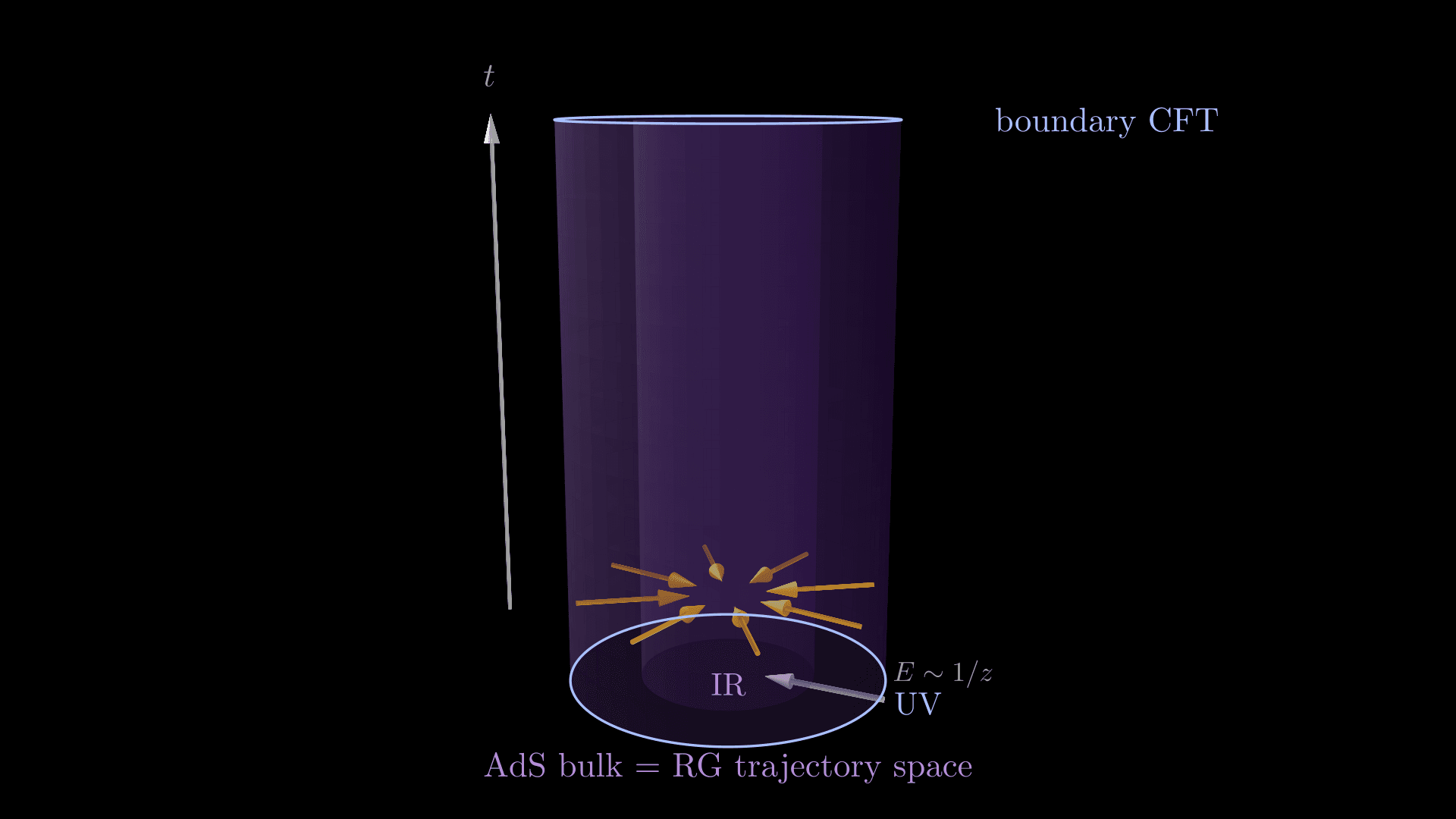
Moving from the boundary into the bulk is RG flow. The extra holographic dimension is the energy axis of the boundary theory: large radius corresponds to UV (high energy), small radius to IR (low energy), with relating bulk depth to boundary energy scale. The eight inward arrows show RG trajectories at a single time slice — at every other slice the same picture holds, since AdS is translation-invariant in .
The duality generalizes: M-theory on is dual to the 6D theory, providing a holographic window into a theory that would otherwise be inaccessible. The correspondence has been used in theoretical physics and in applied holographic calculations across condensed matter, heavy-ion collisions, and black hole information.
Topological twists
The last avatar of SUSY worth naming connects the entire story back to pure mathematics.
In 1988 Witten ("Topological quantum field theory," Comm. Math. Phys. 117, 353) took an super-Yang-Mills theory in 4D and redefined the Lorentz group by mixing it with the R-symmetry:
What this means concretely: the Lorentz group in 4D Euclidean signature factors as . Witten's twist replaces one of these factors with the diagonal subgroup of and the R-symmetry — the set of pairs with the same group element acting on both sides. Under this redefined Lorentz group, the supercharges (which originally transformed as spinors) decompose into a vector plus a scalar plus an antisymmetric tensor. The scalar piece is a Lorentz scalar globally on any oriented 4-manifold, with no spin-structure required. That scalar is the BRST-like operator .
One of the supercharges therefore becomes a Lorentz scalar nilpotent operator with , now globally well-defined on any oriented 4-manifold. Restricting observables to the cohomology of eliminates local degrees of freedom and leaves a topological sector. Cohomology of a nilpotent operator : the space of -closed states () modulo -exact states (). The familiar example is de Rham cohomology, where is the exterior derivative; closed forms modulo exact forms are the topological invariants of the manifold. The same construction here strips out everything that is not topologically meaningful.
The path integral on a 4-manifold then localizes to the moduli space of instantons on . Instantons are finite-action solutions of the Euclidean Yang-Mills equations — localized "lumps" of gauge field with quantized topological charge. Their moduli space is the space of all such solutions modulo gauge equivalence; for on , the -instanton moduli space has dimension . The path integral of the topologically twisted theory localizes from an infinite-dimensional integral over all gauge fields to a finite-dimensional integral over this moduli space. The resulting topological invariants are precisely the Donaldson polynomial invariants of — integer-valued invariants of smooth 4-manifolds, sensitive enough to distinguish manifolds that are homeomorphic but not diffeomorphic (the famous exotic 's). They were defined by Simon Donaldson in 1982 by counting solutions to the anti-self-dual Yang-Mills equation; Witten's twist showed they are physics observables of a topological QFT.
This earned Witten the Fields Medal in 1990 (the only physicist ever to receive it).
Later work compounded the connection. Kapustin and Witten (hep-th/0604151, 2006) took a different twist of SYM and compactified on a Riemann surface. The S-duality of the gauge theory becomes the geometric Langlands correspondence. The Langlands program is a network of conjectures relating number theory, representation theory, and harmonic analysis; geometric Langlands is its avatar over algebraic curves rather than number fields. Loosely: representations of the fundamental group of a Riemann surface in a Lie group correspond to certain -modules on a moduli space attached to the Langlands dual group . Kapustin and Witten showed this duality is the S-duality of SYM — the same physics that runs strong-coupling-to-weak-coupling, applied to a different observable, becomes a deep correspondence in pure mathematics. Seiberg and Witten (1994, hep-th/9407087) used a related twist to solve gauge theory, producing the Seiberg-Witten equations that replaced Donaldson theory as the practical tool in 4-manifold topology.
The pattern: SUSY + R-symmetry + mixing one into the other = the topology of the underlying manifold falls out of the gauge theory. The path integral, which once seemed impossibly complex, localizes to finite-dimensional moduli spaces.
Where things stand
SUSY has not been found at the LHC. Stops lighter than TeV and gluinos lighter than TeV are excluded in simplified-model searches; the pMSSM picture (the phenomenological MSSM, a restricted-parameter version of the full MSSM with simplifying assumptions about flavor and CP that reduce the parameter space from over a hundred to about twenty) is more nuanced but also more constrained than pre-LHC expectations. If the stop is near TeV, the residual contribution to is already one to two orders of magnitude larger than itself, and the cancellation now requires percent-level fine-tuning — not the of the pure SM, but a tuning all the same. The naturalness argument is weakened, and whether SUSY is wrong or just sits at a higher scale, we do not know.
What survives the LHC null results is the algebraic structure. Coleman-Mandula says no bosonic extension of Poincaré is possible; HLS says the unique fermionic loophole is supersymmetry. Supersymmetry, in turn, demands superspace, and Nahm says superconformal symmetry has a hard ceiling at . The 4D and 6D theories at that ceiling are among the richest structures in all of QFT — AdS/CFT connects them to a gravitational bulk, and topological twisting connects them to pure mathematics.
The "extra dimensions" of the title are real in three distinct senses, none of them metaphor:
- Superspace: the SUSY algebra has nowhere to act on ordinary spacetime alone; adjoining anticommuting Grassmann coordinates is geometrically forced, not optional. You cannot write down SUSY transformations without it.
- Spatial extra dimensions: 10D string theory and 11D M-theory require additional compact directions, and the shape of those directions (Calabi-Yau, ) determines how much SUSY survives in 4D. These are the natural habitat for the theories with maximum SUSY.
- The holographic dimension: in AdS/CFT, the radial direction of the bulk is the energy axis of the boundary CFT. RG flow is literally motion in the extra dimension; the geometry emerges from the field theory.
Whether any of these correspond to physical reality at scales we will probe is a separate question, and one we cannot currently answer. But the structure is there whether or not a stop turns up at the next collider.
For further reading: David Tong's Cambridge SUSY notes and String Theory notes are free, precise, and pedagogically excellent. The Martin SUSY Primer (arXiv:hep-ph/9709356) is the standard reference for phenomenological SUSY. For the algebraic side, Nahm's original paper (Nucl. Phys. B135, 1978) and the Cordova-Dumitrescu-Intriligator review (arXiv:1612.00809) are the cleanest sources.
Comments